Information Retrieval on the COVID-19 Open Research Dataset (CORD-19) Part one: TF-IDF and Cosine Similarity

Scenario

In response to the COVID-19 pandemic, the White House and a coalition of leading research groups have prepared the COVID-19 Open Research Dataset (CORD-19). CORD-19 is a resource of over 181,000 scholarly articles, including over 80,000 with full text, about COVID-19, SARS-CoV-2, and related coronaviruses. This freely available dataset is provided to the global research community to apply recent advances in Information Retrieval and other AI techniques to generate new insights in support of the ongoing fight against this infectious disease. There is a growing urgency for these approaches because of the rapid acceleration in new coronavirus literature, making it difficult for the medical research community to keep up.

The task

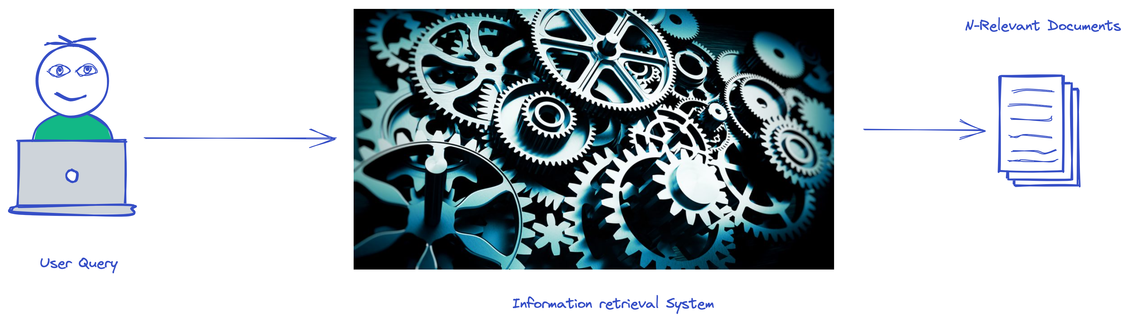
For this tutorial, we will write an Information Retrieval pipeline that helps anyone to query the cord-19 dataset and find relevant articles for their queries.

We will show two different approaches to building that pipeline. The first approach uses the TF-IDF and cosine similarity between the query and the articles. We will use Elasticsearch with the python API to search our articles for the second one.

For the first step, we will leverage the TF-IDF vectorizer from Sklearn. In contrast, for the second one, we will leverage the python elastic search dsl. If you are familiar with ORMs, this library is like an object-relational framework to interact with the elastic search database. If you have a background in python and some NLP experience, this is a fantastic tool for a smooth interaction with elastic search.

This series is a part of an assignment I did for my Information Retrieval course. I decided to publish it online because of the lack of relevant tutorials on this topic.

This will be a two parts tutorial.

For the first part:

Data Collection: In this section, we will go through downloading the dataset from Kaggle and saving it as a csv file.
Data Cleaning: We will pre-process and clean the text.
Keyword selection: We will use TF-IDF to find the appropriate keywords for each document.
Querying : In this section we will query the article using TF-IDF.

For the second part:

Model Creation and Indexing: We will build our elastic search model and create our index in the database.
Querying: We will show to perform some simple queries on our database and preprocess the results.

For this series, I am assuming the following:

You have elastic-search installed and running on your computer.
You have Python 3.7 installed.
You are familiar with the basics of text processing in Python and Object-Relational Mapping(ORM).

If that is the case for you, let’s get started.

Data Collection

In this section, we will go through downloading the dataset from Kaggle and how to process it in chunks.

The dataset is huge, and for this tutorial, we will use only the metadata release alongside the dataset.

Downloading the metadata file

The simplest way to download the data is to head to the competition link then select the metadata.csv file, and finally, click on the download button to download it and save it in a place in your local machine.

The data comes as a zip file; you will have to unzip it to start using it.

Reading the dataset with Dask.

The dataset is huge. It has more than 1.5Gb. We will use dask and pandas to read the file to make our life easier.

Make sure to have dask and pandas installed in your environment for this project.

With the file downloaded in your local machine, dask and pandas installed, let us write the first code to read the dataset.

import  pandas  as  pd
from  pathlib  import  Path
import  dask.dataframe  as  dd
import  numpy  as  np

If the libraries are well imported, let us read the file.

DATA_PATH = Path.cwd().joinpath("data")
metadata_path = DATA_PATH.joinpath("metadata.csv")
data = dd.read_csv(metadata_path,  dtype={"pubmed_id":  np.object0,  'arxiv_id':  'object',  'who_covidence_id':  'object'})

Those lines, call the read_csv from function from dask to read the file and specify some columns data mapping. Under the assumption that you have a data folder on the same level as this jupyter notebook and it is named metadata.csv. If that is not the case , you can pass the exact path of your csv file to the read_csv function.

Why is Dask faster than Pandas?

Remember, we are dealing with a large dataset. Pandas would like to load the whole data in memory. But for a small computer, 1.7 Gb is a lot of data to fit in memory, which would take us a lot of time.

A workaround for this problem would be to read our dataset in different chunks with pandas. Dask is doing almost the same, it read the dataset in parallel using chunk but transparently for the end users.

It avoids us writing a lot of code that will read the data in chunks, process each chunk in parallel, and combine the whole data in one dataset. Check this tutorial here for more details about how dask is faster than pandas.

Once our data is read, let us select a subset for our tutorial.

important_columns = ["pubmed_id",  "title",  "abstract",  "journal",  "authors",  "publish_time"]

The dataset has 59k rows but for this exercice will will only work this the a sample of 1000 rows which is roughly the 1/60 of the whole dataframe

sample_df = data.sample(frac=float(1/300))
sample_df = sample_df.dropna(subset=important_columns)
sample_df = sample_df.loc[:,  important_columns]

We are still using a dask dataframe; let us convert it to a pandas dataframe.

data_df = sample_df.compute()

This line creates the pandas dataframe we will be working with for the rest of the tutorial. The bellow lines will drop null values in the abstract of the dataset and

data_df  =  data_df.dropna(subset=['abstract'],  axis="rows")
data_df  =  data_df.set_index("pubmed_id")
data_df.head()

pubmed_id	title	abstract	journal	authors	publish_time
32165633	Acid ceramidase of macrophages traps herpes si…	Macrophages have important protective function…	Nat Commun	Lang, Judith; Bohn, Patrick; Bhat, Hilal; Jast…	2020-03-12
18325284	Resource Allocation during an Influenza Pandemic	Resource Allocation during an Influenza Pandemic	Emerg Infect Dis	Paranthaman, Karthikeyan; Conlon, Christopher …	2008-03-01
30073452	Analysis of pig trading networks and practices…	East Africa is undergoing rapid expansion of p…	Trop Anim Health Prod	Atherstone, C.; Galiwango, R. G.; Grace, D.; A…	2018-08-02
35017151	Pembrolizumab and decitabine for refractory or…	BACKGROUND: The powerful ‘graft versus leukemi…	J Immunother Cancer	Goswami, Meghali; Gui, Gege; Dillon, Laura W; …	2022-01-11
34504521	Performance Evaluation of Enterprise Supply Ch…	In order to make up for the shortcomings of cu…	Comput Intell Neurosci	Bu, Miaoling	2021-08-30

The dataframe contains the following columns :

The pub med id is a unique id to identify the article.

Title: the title of the research paper
authors: the author of the paper
publish time: the date the paper was published The abstract is the abstract of the paper, which is the text we will use for indexing purposes for this work. With our pandas dataset in place, let us move to the next part: text processing.

Text Processing

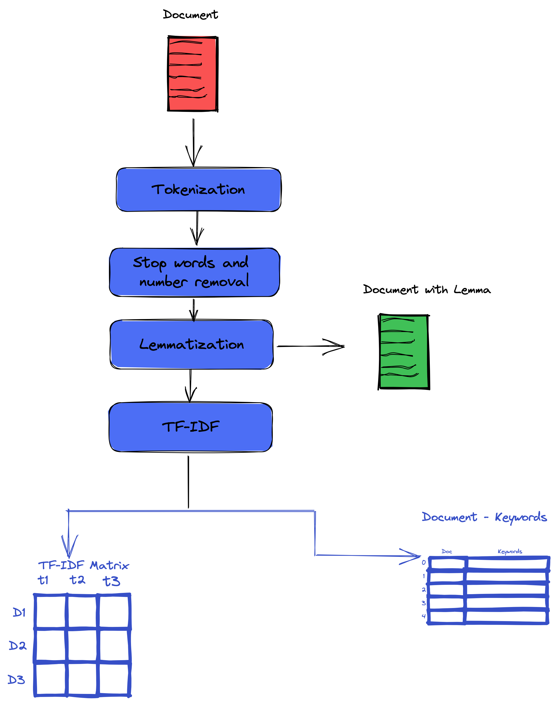
In this part, we will perform text processing. Our input is the raw text for the paper abstract for this section. Our output is the cleaned version of the input text. Our preprocessing consists of the following steps: tokenization, lemmatization, stop word removal, lowercasing, special characters, and number removal.

For this step, we will be using Spacy,NLTK, and regular expressions to perform our preprocessing. Ensure you have spacy and NLTK installed before running the code in this section. Check also if you have installed the en_core_web_sm package. If not install it from this link

import  spacy
import  nltk
import  re
nlp = spacy.load('en_core_web_sm')
stopwords_list = nltk.corpus.stopwords.words('english')

Tokenization

Tokenization is the process of splitting a document into tokens, basically splitting a bunch of text into words. Spacy has a built-in tokenizer that helps us with this.

Stopwords removal.

Stop words are words that have no special significance when analyzing the text. Those words are frequent in the corpus but are useless for our analysis and example of them are a, an, the, and the like.

The following function will perform stop word removal for us :

def  remove_stopwords(text,  is_lower_case=False):
    tokens  =  nltk.word_tokenize(text)
    tokens  =  [token.strip() for token in tokens]
    if is_lower_case:
        filtered_tokens = [token  for  token  in  tokens  if  token  not  in  stopwords_list]
    else:
        filtered_tokens  =  [token  for  token  in  tokens  if  token.lower()  not  in  stopwords_list]
    filtered_text  =  '  '.join(filtered_tokens)
    return  filtered_text

Special characters and number removal.

Special characters and symbols are usually non-alphanumeric or occasionally numeric characters which add extra noise in unstructured text. For our problem, since our corpus is built with articles from the biomedical field, there are a lot of numbers denoting quantities and dosages. We have decided to remove them to simplify the tutorial.

Lematization

In this step, we will use lemmatization instead of stemming,

Chirstopher Maning define lemmatization as :

Lemmatization usually refers to doing things properly with the use of a vocabulary and morphological analysis of words, normally aiming to remove inflectional endings only and to return the base or dictionary form of a word, which is known as the lemma . If confronted with the token saw, stemming might return just s, whereas lemmatization would attempt to return either see or saw depending on whether the use of the token was as a verb or a noun. The two may also differ in that stemming most commonly collapses derivationally related words, whereas lemmatization commonly only collapses the different inflectional forms of a lemma.

A good lemmatizer will replace words such as foot by feet; chosen, choose, by choice.; etc.

This approach has some advantages because it will help not spread the information between different word forms derived from the same lemma. Therefore, it will lead to an accurate TF-IDF because the same semantic information is assembled in one place.

The code for lemmatization is as follow :

def  lemmatize_text(text):
    text  =  nlp(text)
    text  =  '  '.join([word.lemma_  if  word.lemma_  !=  '-PRON-'  else  word.text  for  word  in  text])
    return  text

Finally, we apply the preprocessing function to our dataset to generate a cleaned version for each abstract.

def preprocess_text(text,  text_lower_case=True,  text_lemmatization=True, stopword_removal=True):  
    if text_lower_case:
        text = text.lower().strip()
    
    text = re.sub(r'[^\w\s]', '', text)
    text = re.sub(r'[\r|\n|\r\n]+', ' ',text)
    text = re.sub(r'\d+', '', text)
    if text_lemmatization:
        text = lemmatize_text(text)
    text = re.sub(' +', ' ', text)
        # remove stopwords
    if stopword_removal:
        text = remove_stopwords(text, is_lower_case=text_lower_case)
    return text

data_df['abstract_cleaned']  =  data_df['abstract'].apply(preprocess_text)

With our text cleaned, we can move to our tutorial’s next section, which generates the most relevant keywords for each abstract.

Keyword Generation using Term Inverse - Document Frequency (Tf-IDF)

To generate keywords for each paper, we have to find a heuristic that finds the most relevant words while penalizing the common phrase in our corpus. Practitioners have widely used the Term Frequency-Inverse Document Frequency (TF-IDF) to generate important keywords in documents in Information Retrieval. But what is TF-IDF? It combines two metrics, the Term frequency and the Inverse Document Frequency.

Term Frequency

[K. Sparck Jones.] defines the term frequency (TF) as a numerical statistic that reflects how important a word is to document in a collection or a corpus. It is the relative frequency of term w within the document d.

It is computed using the following formula :

\[\begin{equation} tf(w,d) = \frac{f_{w,d}}{\sum_{t\ast}^{d}f_{w\ast,d}} \end{equation}\]

with \(f_{w,d}\) defined as the raw count of the word w in the document d, and \(\sum_{t\ast}^{d}f_{w\ast,d}\) as the total number of terms in document d (counting each occurrence of the same term separately).

Inverse Document Frequency

The inverse document frequency is defined as the log of the ratio between the total number of documents in the corpus and the number of documents with the word. It is a measure the amount of information provided by the word. \(\begin{equation} idf(w, d) = log\frac{N}{1 + (\left | d \in D : w \in d \right |)} \end{equation}\) with

N: total number of documents in the corpus N and the denominator represent the number of documents with the word w. This helps to penalize the most common word in a corpus. Those words carry fewer values for in the corpus.

For the curious who want to know why we use the log in the IDF, check out this answer from StackOverflow.

The TF-IDF combines both the Term Frequency and the Inverse Document Frequency.

\[(tf_idf)_{t,d} = Idf_t * TF_{w, d}\]

Applying TF-IDF to our corpus

To apply TF-IDF we will leverage the sklearn implementation of the algorithm. Before running the bellow code, make sure you have sklearn installed.

If the sklearn is installed, you can import it with the bellow code.

from  sklearn.feature_extraction.text  import  TfidfVectorizer

def create_tfidf_features(corpus, max_features=10000, max_df=0.95, min_df=2):
    """ Creates a tf-idf matrix for the `corpus` using sklearn. """
    tfidf_vectorizor = TfidfVectorizer(decode_error='replace', strip_accents='unicode', analyzer='word', 
                                       stop_words='english', ngram_range=(1, 3), max_features=max_features, 
                                       norm='l2', use_idf=True, smooth_idf=True, sublinear_tf=True,
                                       max_df=max_df, min_df=min_df)
    X = tfidf_vectorizor.fit_transform(corpus)
    print('tfidf matrix successfully created.')
    return X, tfidf_vectorizor

This article recommended to use TfidfVectorizer with smoothing (smooth_idf = True) and normalization (norm='l2") turned on. These parameters will better account for text length differences and produce more meaningful to–IDF scores. Smoothing and L2 normalization are the default settings for TfidfVectorizer,` so you don’t need to include any extra code at all to turn them on.

On top of the smoth_idf and norm hyperparameters, the other keys hyperparameters are :

max_features which denotes the max number of words to keep in our vocabulary
max_df: When building the vocabulary, ignore terms that have a document frequency strictly higher than the given threshold
min_df: When building the vocabulary, ignore terms that have a document frequency strictly lower than the given threshold. This value is also called a cut-off in the literature.
n_gram_range is the number of n-grams to consider when building our vocabulary; for this task, we consider nonograms, bigrams, and trigrams.

data_df = data_df.reset_index()

tf_idf_matrix, tf_idf_vectorizer = create_tfidf_features(data_df['abstract_cleaned'])

After applying the tf_if vectorizer on to our corpus, it will result in the following two objects :

The tf_ifd matrix , is a matrix where rows are the documents and columns are the words in our vocabulary.
The tf_idf_vectorizer is an object that will help us to transform a new document to the TF-IDF version.

The value at the ith row and jth column is the TF-IDF score of the word j in document i.

For better analysis we converted the tf_idf_matrix into a pandas dataframe using the following code :

tfidf_df  =  pd.DataFrame(tf_idf_matrix.toarray(), columns=tf_idf_vectorizer.get_feature_names(), index=[data_df.index])

The next step is to generate the top 20 keywords for each document, those word are the word with the highest tf-idf score within the document.

Before doing that, let’s reorganize the DataFrame so that the words are in rows rather than columns.

tfidf_df = tfidf_df.sort_index().round(decimals=2)
tfidf_df_stacked = tfidf_df.stack().reset_index()
tfidf_df_stacked = tfidf_df_stacked.rename(columns={0:'tfidf','level_1': 'term', "level_0": "doc_id"})

We sort by document and tfidf score and then groupby document and take the first 20 values. Once we have sorted and find the top keywords we can save them in a dictionary where the keys are the the document id and the values are the another dictionary of the term and their tf-idf score.

tfidf_df_stacked  =  tfidf_df_stacked.reset_index().rename(columns={'level_1':'term'})
document_tfidf  =  tfidf_df_stacked.groupby(['doc_id']).apply(lambda  x:  x[['term',  "tfidf"]].set_index("term").to_dict().get('tfidf'))

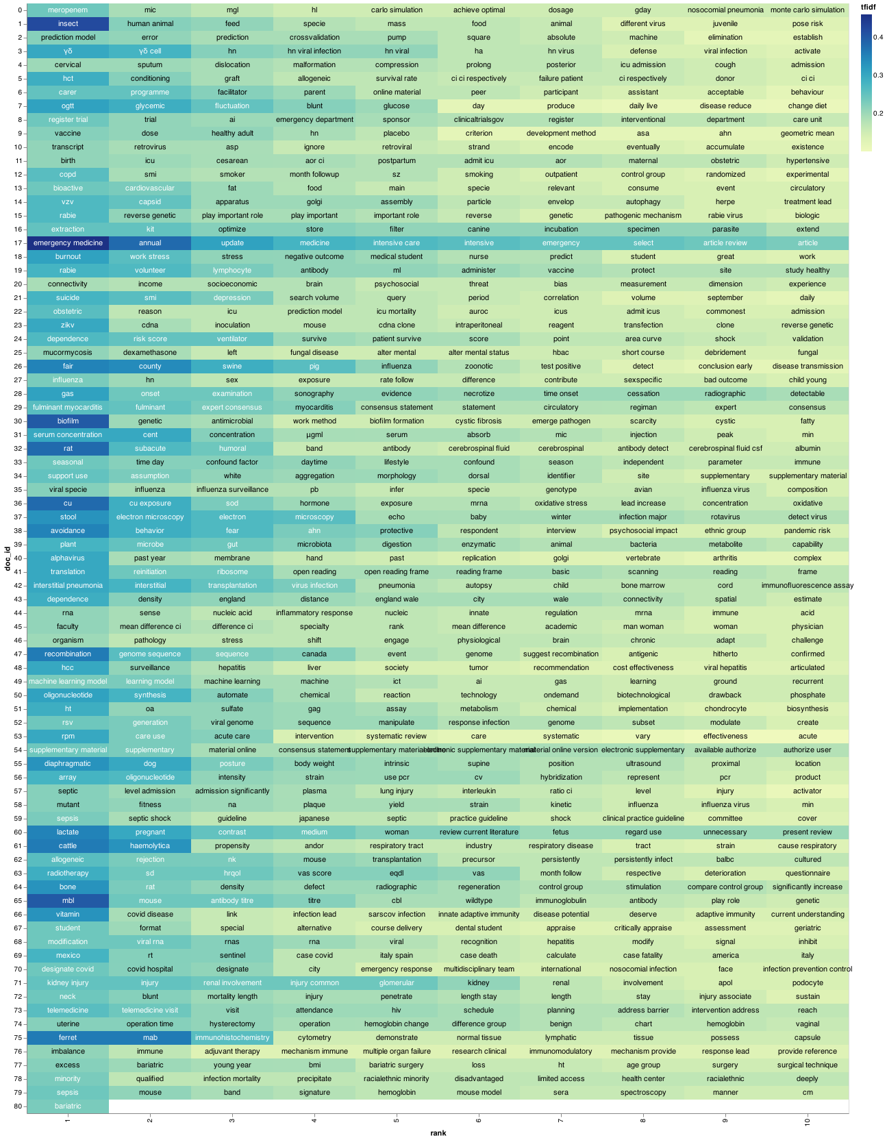
With our documents and the top keyword mappings, we can now visualize what our corpus looks like to have an idea on each paper on the document.

I recently come across a good piece of code that makes visualization for a document using TF-IDF.

I grabbed it from this article.

import altair as alt
import numpy as np

# Terms in this list will get a red dot in the visualization
term_list = ["covid", 'traitement', 'ebola']

# adding a little randomness to break ties in term ranking
top_tfidf_plusRand = tfidf_df_stacked.loc[:800]
top_tfidf_plusRand['tfidf'] = top_tfidf_plusRand['tfidf'] + np.random.rand(tfidf_df_stacked.loc[:800].shape[0])*0.0001

# base for all visualizations, with rank calculation
base = alt.Chart(top_tfidf_plusRand).encode(
    x = 'rank:O',
    y = 'doc_id:N'
).transform_window(
    rank = "rank()",
    sort = [alt.SortField("tfidf", order="descending")],
    groupby = ["doc_id"],
)

# heatmap specification
heatmap = base.mark_rect().encode(
    color = 'tfidf:Q'
)

# red circle over terms in above list
circle = base.mark_circle(size=100).encode(
    color = alt.condition(
        alt.FieldOneOfPredicate(field='term', oneOf=term_list),
        alt.value('red'),
        alt.value('#FFFFFF00')        
    )
)

# text labels, white for darker heatmap colors
text = base.mark_text(baseline='middle').encode(
    text = 'term:N',
    color = alt.condition(alt.datum.tfidf >= 0.23, alt.value('white'), alt.value('black'))
)

# display the three superimposed visualizations
(heatmap + circle + text).properties(width = 1200)

Querying using tf-idf

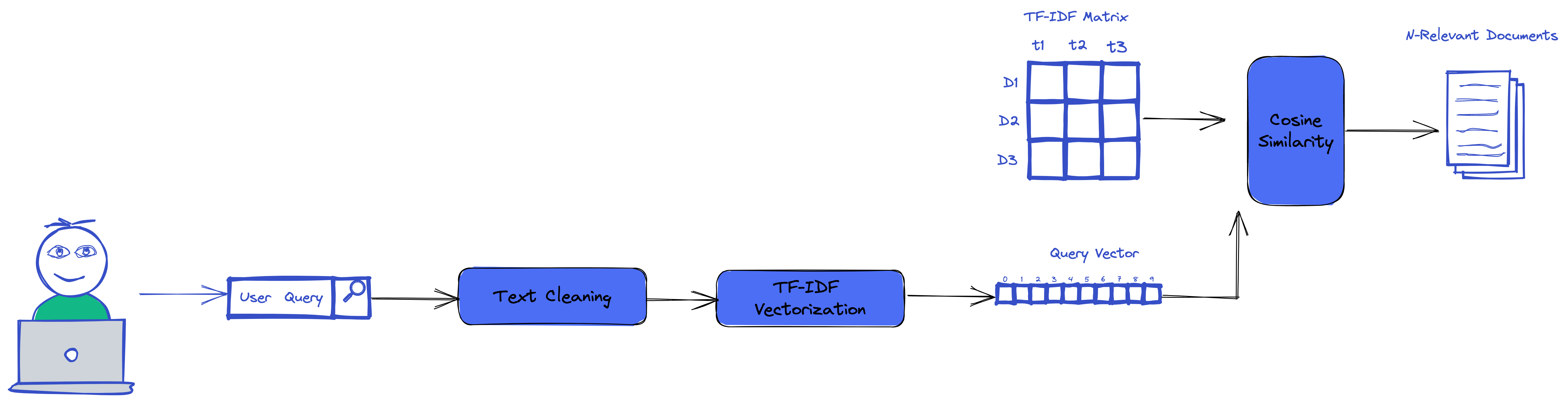
With our TF-IDF we could easily use it to run search and make queries that use the TF-IDF score and cosine similarty.

from sklearn.metrics.pairwise import cosine_similarity

def calculate_similarity(query, X=tf_idf_matrix, vectorizor=tf_idf_vectorizer, top_k=5):
    """ Vectorizes the `query` via `vectorizor` and calculates the cosine similarity of
    the `query` and `X` (all the documents) and returns the `top_k` similar documents.
    """

    # Vectorize the query to the same length as documents
    query_vec = vectorizor.transform(query)
    # Compute the cosine similarity between query_vec and all the documents
    cosine_similarities = cosine_similarity(X, query_vec).flatten()
    # Sort the similar documents from the most similar to less similar and return the indices
    most_similar_doc_indices = np.argsort(cosine_similarities, axis=0)[:-top_k-1:-1]
    return (most_similar_doc_indices, cosine_similarities)

def show_similar_documents(df, cosine_similarities, similar_doc_indices):
    """ Prints the most similar documents using indices in the `similar_doc_indices` vector."""
    counter = 1
    for index in similar_doc_indices:
        print('Top-{}, Similarity = {}'.format(counter, cosine_similarities[index]))
        pubmed_id = df.loc[index]['pubmed_id']
        print('the pubmed id : {}, '.format(pubmed_id))
        print('title {}'.format(data_df.loc[index, "title"]))
        print("abstract {}".format(data_df.loc[index, "abstract"][:50]))
        counter += 1
        print(10 * '**==')

The above code, get our new query, generate it TF-IDF vector. Then it computes the cosine similarity between the vectors and all our documents in the TF-IDF matrix.

As the result, it returns the top n rows in the matrix which are similar to our query vector.

Let us try to check how it works in practice.

import time
query = ['are gorillas responsible of ebola']
search_start = time.time()
sim_vecs, cosine_similarities = calculate_similarity(query)
search_time = time.time() - search_start
print("search time: {:.2f} ms".format(search_time * 1000))
print()
show_similar_documents(data_df, cosine_similarities, sim_vecs)

search time: 7.60 ms

Top-1, Similarity = 0.25484833157402037
the pubmed id : 32287784, 
title Wuhan virus spreads
abstract We now know the virus responsible for deaths and i
**==**==**==**==**==**==**==**==**==**==
Top-2, Similarity = 0.2332808978421972
the pubmed id : 32162604, 
title How Is the World Responding to the Novel Coronavirus Disease (COVID-19) Compared with the 2014 West African Ebola Epidemic? The Importance of China as a Player in the Global Economy
abstract This article describes similarities and difference
**==**==**==**==**==**==**==**==**==**==
Top-3, Similarity = 0.1286925639778678
the pubmed id : 19297495, 
title Aquareovirus effects syncytiogenesis by using a novel member of the FAST protein family translated from a noncanonical translation start site.
abstract As nonenveloped viruses, the aquareoviruses and or
**==**==**==**==**==**==**==**==**==**==
Top-4, Similarity = 0.11561157619559267
the pubmed id : 27325914, 
title Consortia critical role in developing medical countermeasures for re-emerging viral infections: a USA perspective.
abstract Viral infections, such as Ebola, severe acute resp
**==**==**==**==**==**==**==**==**==**==
Top-5, Similarity = 0.10755790364315998
the pubmed id : 33360484, 
title Neuropathological explanation of minimal COVID-19 infection rate in newborns, infants and children – a mystery so far. New insight into the role of Substance P
abstract Sars-Cov-2 or Novel coronavirus infection (COVID-1
**==**==**==**==**==**==**==**==**==**==

That is all for the first part of this tutorial , We have learned how to build TF-IDF vectors, and how to leverage the cosine similarity to compute and retrieve documents that matches a query. In the second part of the tutorial we will learn how to use elasticsearch to perform the same task.